1_DE gene analysis
Yang & Steve
24/02/2020
Last updated: 2020-10-28
Checks: 6 1
Knit directory: 20190717_Lardelli_RNASeq_Larvae/
This reproducible R Markdown analysis was created with workflowr (version 1.6.0). The Checks tab describes the reproducibility checks that were applied when the results were created. The Past versions tab lists the development history.
The R Markdown file has unstaged changes. To know which version of the R Markdown file created these results, you’ll want to first commit it to the Git repo. If you’re still working on the analysis, you can ignore this warning. When you’re finished, you can run wflow_publish to commit the R Markdown file and build the HTML.
Great job! The global environment was empty. Objects defined in the global environment can affect the analysis in your R Markdown file in unknown ways. For reproduciblity it’s best to always run the code in an empty environment.
The command set.seed(20200227) was run prior to running the code in the R Markdown file. Setting a seed ensures that any results that rely on randomness, e.g. subsampling or permutations, are reproducible.
Great job! Recording the operating system, R version, and package versions is critical for reproducibility.
Nice! There were no cached chunks for this analysis, so you can be confident that you successfully produced the results during this run.
Great job! Using relative paths to the files within your workflowr project makes it easier to run your code on other machines.
Great! You are using Git for version control. Tracking code development and connecting the code version to the results is critical for reproducibility. The version displayed above was the version of the Git repository at the time these results were generated.
Note that you need to be careful to ensure that all relevant files for the analysis have been committed to Git prior to generating the results (you can use wflow_publish or wflow_git_commit). workflowr only checks the R Markdown file, but you know if there are other scripts or data files that it depends on. Below is the status of the Git repository when the results were generated:
Ignored files:
    Ignored:    .DS_Store
    Ignored:    .Rhistory
    Ignored:    .Rproj.user/
    Ignored:    1_DE-gene-analysis_cache/
    Ignored:    1_DE-gene-analysis_files/
    Ignored:    analysis/.DS_Store
    Ignored:    analysis/.Rhistory
    Ignored:    analysis/.Rproj.user/
    Ignored:    analysis/5_WGCNA_cache/
    Ignored:    data/.DS_Store
    Ignored:    data/0_rawData/.DS_Store
    Ignored:    data/1_trimmedData/.DS_Store
    Ignored:    data/2_alignedData/.DS_Store
    Ignored:    files/
    Ignored:    keggdiagram/.DS_Store
    Ignored:    output/.DS_Store

Untracked files:
    Untracked:  analysis/here::here
    Untracked:  output/DEgenes_with_genotype.csv
    Untracked:  output/GOenrichment_enrichmentTable.csv
    Untracked:  output/black_genes.csv
    Untracked:  output/cyan_genes.csv
    Untracked:  output/green_genes.csv
    Untracked:  output/greenyellow_genes.csv
    Untracked:  output/grey60_genes.csv
    Untracked:  output/lightcyan_genes.csv
    Untracked:  output/purple_genes.csv

Unstaged changes:
    Modified:   analysis/1_DE_gene_analysis.Rmd
    Modified:   analysis/5_WGCNA.Rmd
    Modified:   analysis/6_Variance_Partition_Analysis.Rmd
    Modified:   analysis/index.Rmd

Staged changes:
    Modified:   .RData
    New:        analysis/5_WGCNA.Rmd
    New:        analysis/6_Variance_Partition_Analysis.Rmd
Note that any generated files, e.g. HTML, png, CSS, etc., are not included in this status report because it is ok for generated content to have uncommitted changes.
These are the previous versions of the R Markdown and HTML files. If you’ve configured a remote Git repository (see ?wflow_git_remote), click on the hyperlinks in the table below to view them.
| File | Version | Author | Date | Message |
|---|---|---|---|---|
| Rmd | 075ff49 | yangdongau | 2020-03-12 | Add in description and gene_biotype |
| Rmd | 6c61705 | yangdongau | 2020-02-27 | Compiled DE Gene analysis |
| html | 6c61705 | yangdongau | 2020-02-27 | Compiled DE Gene analysis |
Setup
library(limma)
library(edgeR)
library(AnnotationHub)
library(tidyverse)
library(magrittr)
library(pander)
library(ggrepel)
library(scales)
library(RUVSeq)

theme_set(theme_bw())
panderOptions("big.mark", ",")
panderOptions("table.split.table", Inf)
panderOptions("table.style", "rmarkdown")
if (interactive()) setwd(here::here("analysis"))
# Get GC content and lengths
gcTrans <- url("https://uofabioinformaticshub.github.io/Ensembl_GC/Release96/Danio_rerio.GRCz11.96.rds") %>%
readRDS()
gcGene <- readRDS(here::here("analysis", "gcGene.rds"))Annotation was set up as a EnsDb object based on Ensembl Release 96
ah <- AnnotationHub() %>%
  subset(species == "Danio rerio") %>%
  subset(dataprovider == "Ensembl") %>%
  subset(rdataclass == "EnsDb")
ensDb <- ah[["AH69169"]]
genes <- genes(ensDb)
transGR <- transcripts(ensDb)
cols2keep <- c("gene_id", "gene_name", "gene_biotype", "entrezid","description","entrezid")
mcols(genes) <- mcols(genes)[cols2keep] %>%
  as.data.frame() %>%
  dplyr::select(-entrezid) %>%
  left_join(as.data.frame(mcols(gcGene))) %>%
  distinct(gene_id, .keep_all = TRUE) %>%
  set_rownames(.$gene_id) %>%
  DataFrame() %>%
  .[names(genes),]
genesGR <- genes(ensDb)
Prior to count-level analysis, the initial dataset was pre-processed using the following steps:
- Adapters were removed from any reads
- Bases were removed from the end of reads when the quality score dipped below 30
- Reads < 35bp after trimming were discarded
After trimming alignment was performed using STAR v2.5.3a to the Danio rerio genome included in Ensembl Release 96 (GRCz11). Aligned reads were counted for each gene if the following criteria were satisfied:
- Alignments were unique
- Alignments strictly overlapped exonic regions
minSamples <- 6
minCpm <- 1
counts <- here::here("data", "2_alignedData", "featureCounts", "genes.out") %>%
read_tsv() %>%
set_colnames(basename(colnames(.))) %>%
set_colnames(str_remove(colnames(.), "Aligned.+")) %>%
gather(key = "Library", value = "Counts", -Geneid) %>%
dplyr::mutate(Sample = str_remove_all(Library, "_2")) %>%
group_by(Geneid, Sample) %>%
dplyr::summarise(Counts = sum(Counts)) %>%
tidyr::spread(key = "Sample", value = "Counts") %>%
as.data.frame() %>%
column_to_rownames("Geneid")
genes2keep <- cpm(counts) %>%
is_greater_than(minCpm) %>%
rowSums() %>%
is_weakly_greater_than(minSamples)Counts were then loaded and summed across replicate sequencing runs. Genes were only retained if receiving more than 1 cpm in at least 6 samples. This filtering step discarded 12,661 genes as undetectable and retained 19,396 genes for further analysis.
plotDensities(cpm(counts, log = TRUE), legend = FALSE, main = "a) All genes")
plotDensities(cpm(counts[genes2keep,], log = TRUE), legend = FALSE, main = "b) Retained genes")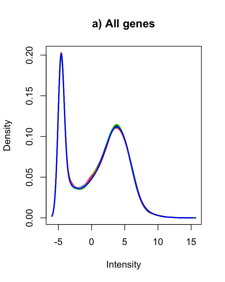
| Version | Author | Date |
|---|---|---|
| 6c61705 | yangdongau | 2020-02-27 |
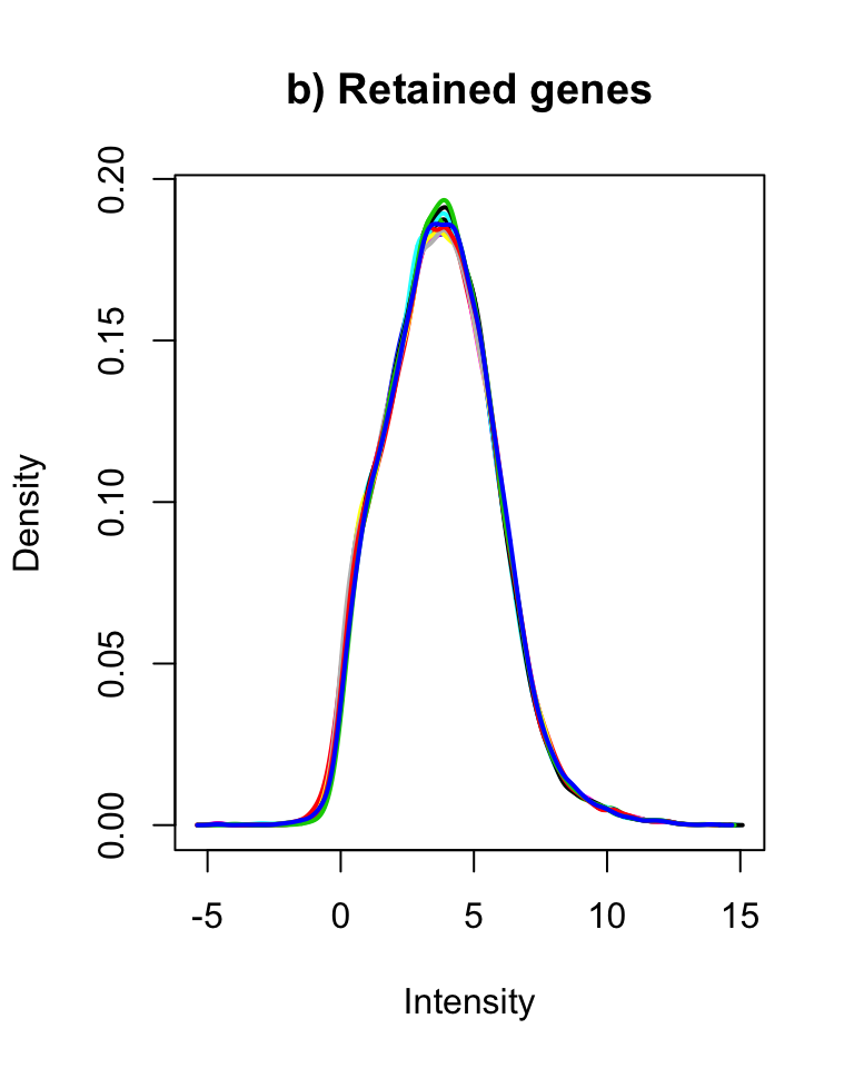
Distribution of logCPM values for a) all and b) retained genes
| Version | Author | Date |
|---|---|---|
| 6c61705 | yangdongau | 2020-02-27 |
dgeList <- counts %>%
  .[genes2keep,] %>%
  DGEList(
    samples = tibble(
      sample = colnames(.),
      group = str_replace_all(sample, "[0-9]*[A-Z]([12])Lardelli", "\\1"),
      pair = str_replace_all(sample, "[0-9]*([A-Z])[0-9].+", "\\1")
    ) %>%
      as.data.frame(),
        genes = genes[rownames(.)] %>%
            as.data.frame() %>%
            dplyr::select(
                ensembl_gene_id = gene_id,
                chromosome_name = seqnames,
                description,
                gene_biotype,
                external_gene_name = gene_name,
                entrez_gene = entrezid.1,
                aveLength,
                aveGc,
                maxLength,
                longestGc
            )
    ) %>%
    calcNormFactors(method = "TMM") %>%
    estimateDisp()
Design matrix not provided. Switch to the classic mode.dgeList$samples$Genotype <- c("Q96K97del/+", "WT")[dgeList$samples$group] %>%
factor(levels = c("WT", "Q96K97del/+"))Counts were then formed into a DGEList object. Library sizes after alignment, counting and gene filtering ranged between 44,498,373 and 52,779,608 reads.
Data Inspection
pca <- dgeList %>%
  cpm(log = TRUE) %>%
  t() %>%
  prcomp()
summary(pca)$importance %>% pander(split.tables = Inf) | PC1 | PC2 | PC3 | PC4 | PC5 | PC6 | PC7 | PC8 | PC9 | PC10 | PC11 | PC12 | |
|---|---|---|---|---|---|---|---|---|---|---|---|---|
| Standard deviation | 21.59 | 17.49 | 13.54 | 12.32 | 11.16 | 10.77 | 10.38 | 10.13 | 9.387 | 7.599 | 7.202 | 4.868e-14 |
| Proportion of Variance | 0.2655 | 0.1742 | 0.1045 | 0.08647 | 0.07089 | 0.06608 | 0.06135 | 0.0585 | 0.05019 | 0.03289 | 0.02955 | 0 |
| Cumulative Proportion | 0.2655 | 0.4396 | 0.5441 | 0.6306 | 0.7015 | 0.7675 | 0.8289 | 0.8874 | 0.9376 | 0.9705 | 1 | 1 |
PCA of all samples.
| Version | Author | Date |
|---|---|---|
| 6c61705 | yangdongau | 2020-02-27 |
DGE Analysis
Design Marix
Next we setup a design matrix using each pool as its own intercept, with the genotype as the common difference, and recalculated the dispersions
expDesign <- model.matrix(~0 + pair + Genotype, dgeList$samples) %>%
  set_colnames(str_replace(colnames(.), pattern = "Genotype.+", "Mutant"))
dgeList %<>%
  estimateGLMCommonDisp(expDesign) %>%
  estimateGLMTagwiseDisp(expDesign)
deGenes <- dgeList %>%
glmFit(expDesign) %>%
glmLRT(coef = "Mutant") %>%
topTags(n = Inf) %>%
as.data.frame() %>%
set_colnames(gsub("ID.", "", colnames(.))) %>%
as_tibble() %>%
mutate(
Sig = FDR < 0.05,
rankstat = -sign(logFC)*log10(PValue)
) %>%
dplyr::select(
ensembl_gene_id, external_gene_name, logFC, logCPM, LR,
PValue, FDR, Sig,aveGc, aveLength, rankstat
) %>%
arrange(PValue)
deGenesSig <- deGenes %>%
dplyr::filter(Sig)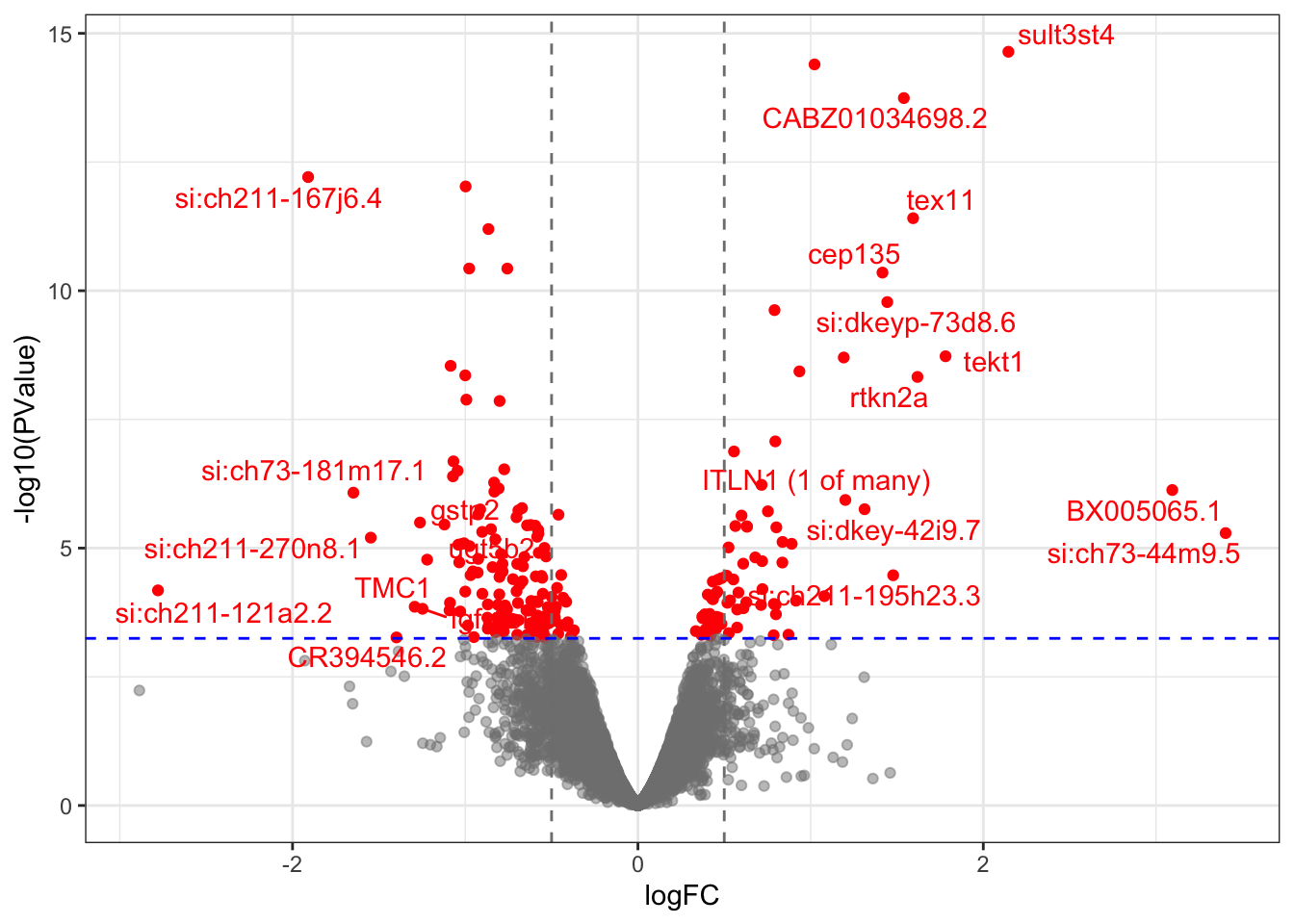
Volcano plot highlighting DE genes. Genes indicated in red were considered as DE, which receive a FDR < 0.05.
| Version | Author | Date |
|---|---|---|
| 6c61705 | yangdongau | 2020-02-27 |
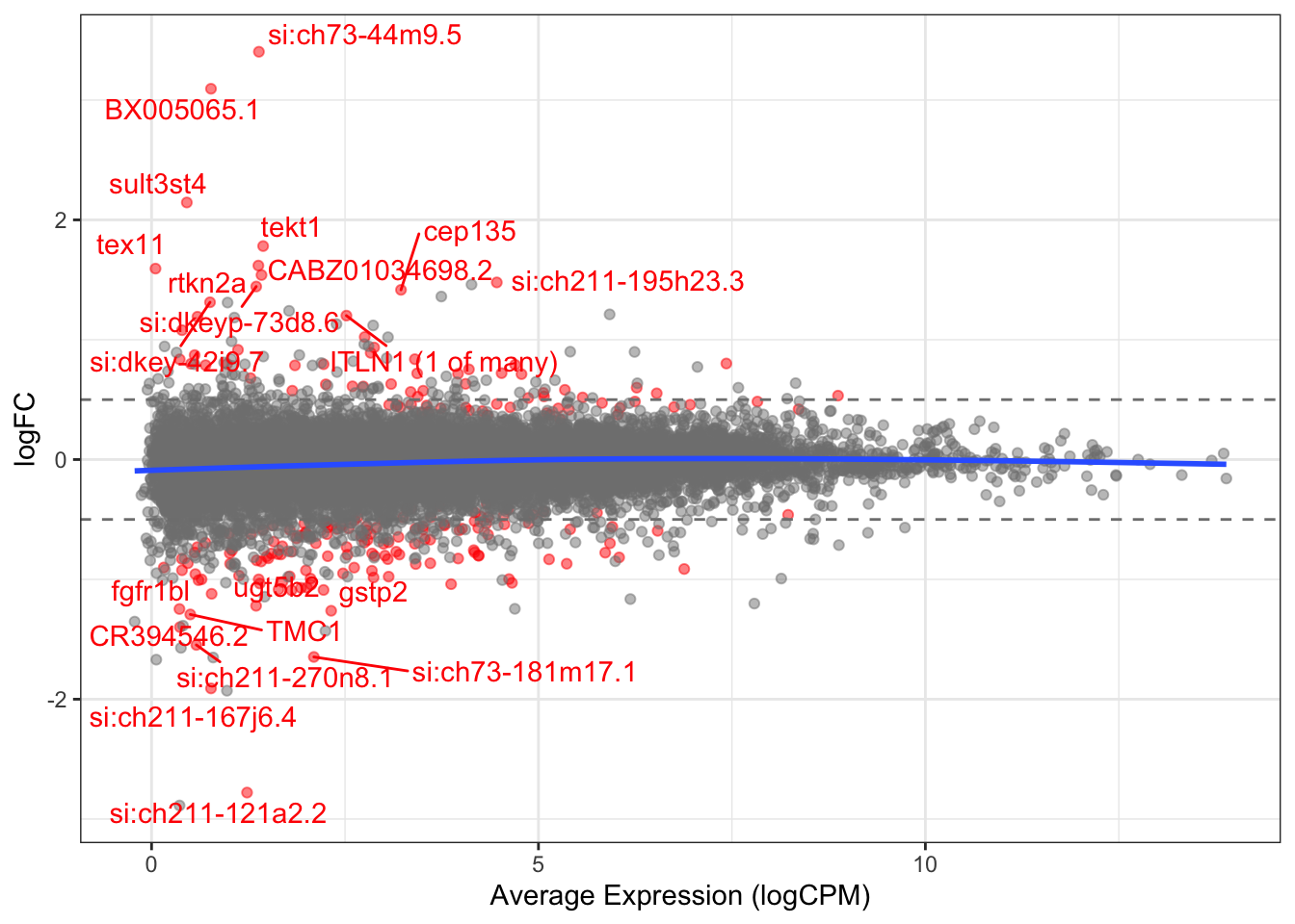
logFC plotted against expression level with significant DE genes shown in red.
| Version | Author | Date |
|---|---|---|
| 6c61705 | yangdongau | 2020-02-27 |
RUV treatment (Remove Unwanted Variation)
Find some ‘unchanged’ genes. Grab the lowest ranked 5000
genes4Control <- deGenes %>%
  arrange(desc(PValue)) %>%
  dplyr::slice(1:5000) %>%
  .[["ensembl_gene_id"]]
length(genes4Control)
[1] 5000k <- 1
ruv <- RUVg(
dgeList$counts,
cIdx = genes4Control,
k = k,
isLog = FALSE,
round = TRUE
)
dgeList$samples <- cbind(dgeList$samples, ruv$W)pcaRUV <- ruv$normalizedCounts %>%
cpm(log = TRUE) %>%
t() %>%
prcomp()
summary(pcaRUV)$importance %>% pander(split.tables = Inf) | PC1 | PC2 | PC3 | PC4 | PC5 | PC6 | PC7 | PC8 | PC9 | PC10 | PC11 | PC12 | |
|---|---|---|---|---|---|---|---|---|---|---|---|---|
| Standard deviation | 17.5 | 13.6 | 12.57 | 11.23 | 10.84 | 10.43 | 10.21 | 9.495 | 7.642 | 7.232 | 0.3216 | 4.41e-14 |
| Proportion of Variance | 0.2344 | 0.1415 | 0.1208 | 0.09644 | 0.08994 | 0.08332 | 0.07973 | 0.069 | 0.0447 | 0.04003 | 8e-05 | 0 |
| Cumulative Proportion | 0.2344 | 0.3759 | 0.4968 | 0.5932 | 0.6831 | 0.7665 | 0.8462 | 0.9152 | 0.9599 | 0.9999 | 1 | 1 |
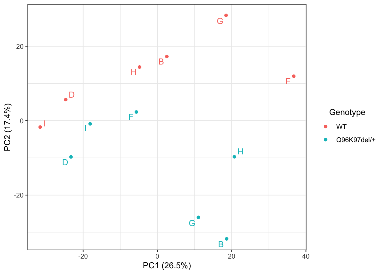
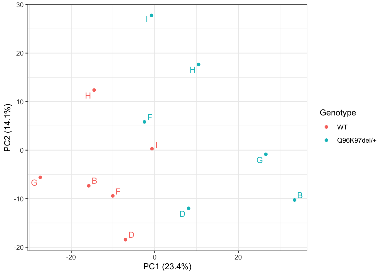
pcaRUV$x %>%
  cbind(dgeList$samples[rownames(.),]) %>%
  ggplot(aes(PC1, PC2, colour = Genotype)) +
  geom_point() +
  geom_text_repel(aes(label = pair), show.legend = FALSE) +
  # stat_ellipse(aes(fill = Genotype), geom = "polygon", alpha = 0.05) +
  xlab(
    paste0(
      "PC1 (", percent(summary(pcaRUV)$importance[2, "PC1"]), ")"
    )
  ) +
  ylab(
    paste0(
      "PC2 (", percent(summary(pcaRUV)$importance[2, "PC2"]), ")"
    )
  )
| Version | Author | Date |
|---|---|---|
| 6c61705 | yangdongau | 2020-02-27 |
expDesignRUV <- model.matrix(~0 + pair + Genotype + W_1, dgeList$samples) %>%
  set_colnames(str_replace(colnames(.), pattern = "Genotype.+", "Mutant"))
Recalculate the dispersions
dgeList %<>%
  estimateGLMCommonDisp(expDesignRUV) %>%
  estimateGLMTagwiseDisp(expDesignRUV)
Now run DE Analysis after RUV
topTable <- dgeList %>%
  glmFit(expDesignRUV) %>%
  glmLRT(coef = "Mutant") %>%
  topTags(n = Inf) %>%
  as.data.frame() %>%
  set_colnames(gsub("ID.", "", colnames(.))) %>%
  as_tibble() %>%
  mutate(
    DE = FDR < 0.01,
    rankstat = -sign(logFC)*log10(PValue)
  ) %>%
  dplyr::select(
    ensembl_gene_id, external_gene_name, description, gene_biotype, logFC, logCPM, LR,
  PValue, FDR, DE,aveGc, aveLength, rankstat
  ) %>%
  arrange(PValue)
topTableDE <- topTable %>%
  dplyr::filter(DE == TRUE)
Check the MA plot
tested <- c("si:ch211-213a13.2", "si:ch211-11p18.6", "mdh1ab", "CABZ01034698.2")
# topTable %>%
topTable %>%
  ggplot(aes(logCPM, logFC)) +
  geom_point(aes(colour = DE), alpha = 0.5) +
  geom_smooth(se = FALSE) +
  geom_hline(yintercept = c(-1, 1)*0.5, linetype = 2) +
  geom_text_repel(
    aes(label = external_gene_name, colour = DE),
    data = . %>%
      dplyr::filter(abs(logFC) > 1.2 & DE | external_gene_name %in% tested),
    show.legend = FALSE
  ) +
  scale_colour_manual(values = c("grey50", "red"))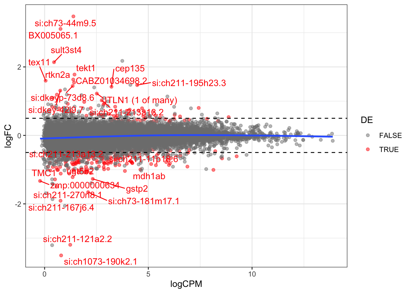
| Version | Author | Date |
|---|---|---|
| 6c61705 | yangdongau | 2020-02-27 |
Check the volcano plot
topTable %>%
  mutate(DE = FDR < 0.01) %>%
  ggplot(aes(logFC, -log10(PValue))) +
  geom_point(aes(colour = DE), alpha = 0.5) +
  geom_vline(xintercept = c(-1, 1)*0.5, linetype = 2) +
  geom_text_repel(
    aes(label = external_gene_name, colour = DE),
    data = . %>%
      dplyr::filter(abs(logFC) > 1.2 & DE | external_gene_name %in% tested),
    show.legend = FALSE
  ) +
  scale_colour_manual(values = c("grey50", "red"))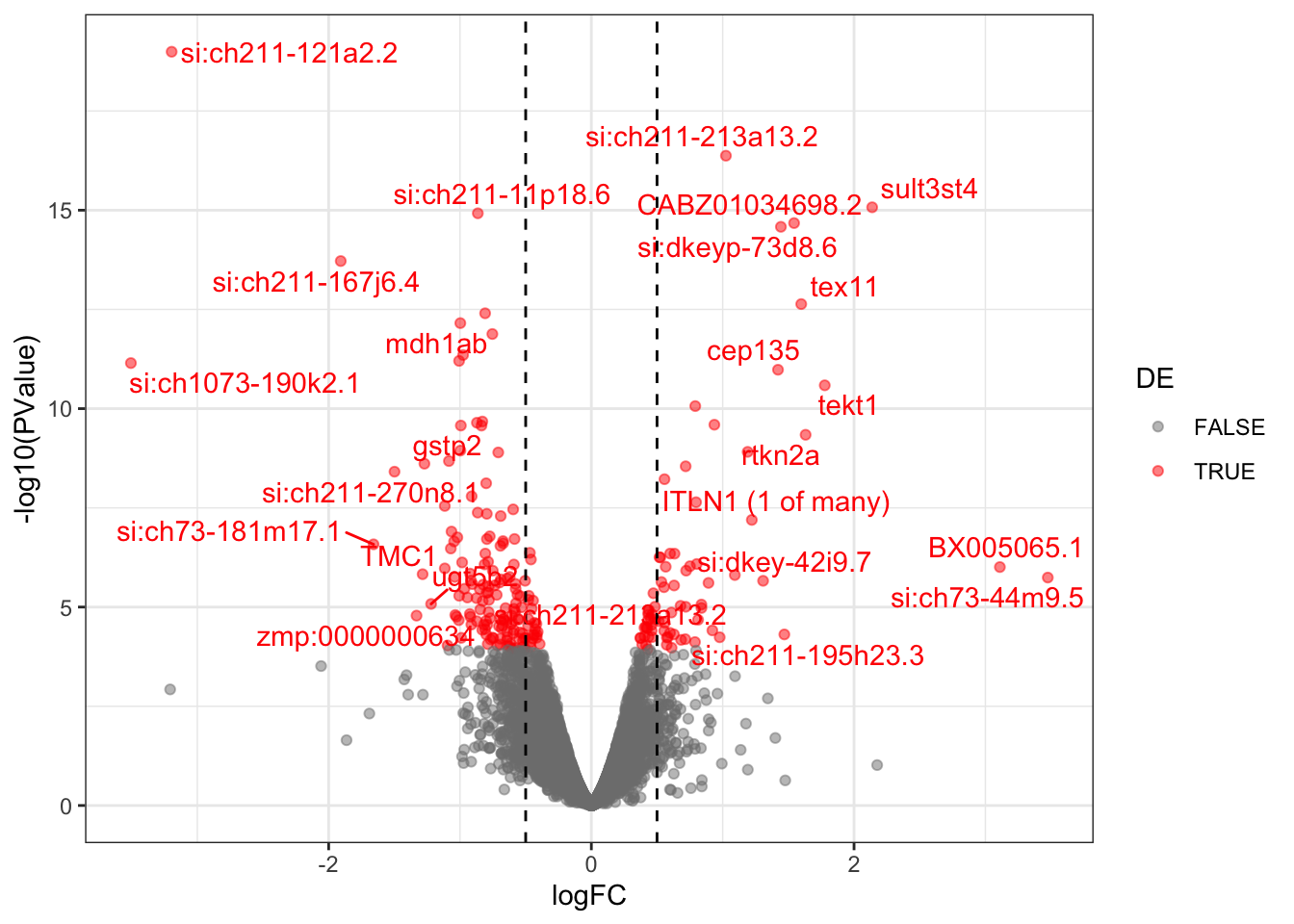
| Version | Author | Date |
|---|---|---|
| 6c61705 | yangdongau | 2020-02-27 |
Compare the two lists
topTable %>%
  dplyr::select(ensembl_gene_id, RUV = logFC, DE) %>%
  left_join(deGenes) %>%
  dplyr::rename(Raw = logFC) %>%
  mutate(
    Status = case_when(
      Sig & DE ~ "Both",
      Sig & !DE ~ "Raw Only",
      !Sig & DE ~ "RUV Only",
      !Sig & !DE ~ "Not DE"
    )
  ) %>%
  ggplot(aes(Raw, RUV,)) +
  geom_point(aes(colour = Status), alpha = 0.5) +
  geom_abline(slope= 1, linetype = 2) +
  geom_vline(xintercept = c(-1, 1)*0.5) +
  geom_hline(yintercept = c(-1, 1)*0.5) +
  scale_colour_manual(values = c("green", "grey50", "red", "blue"))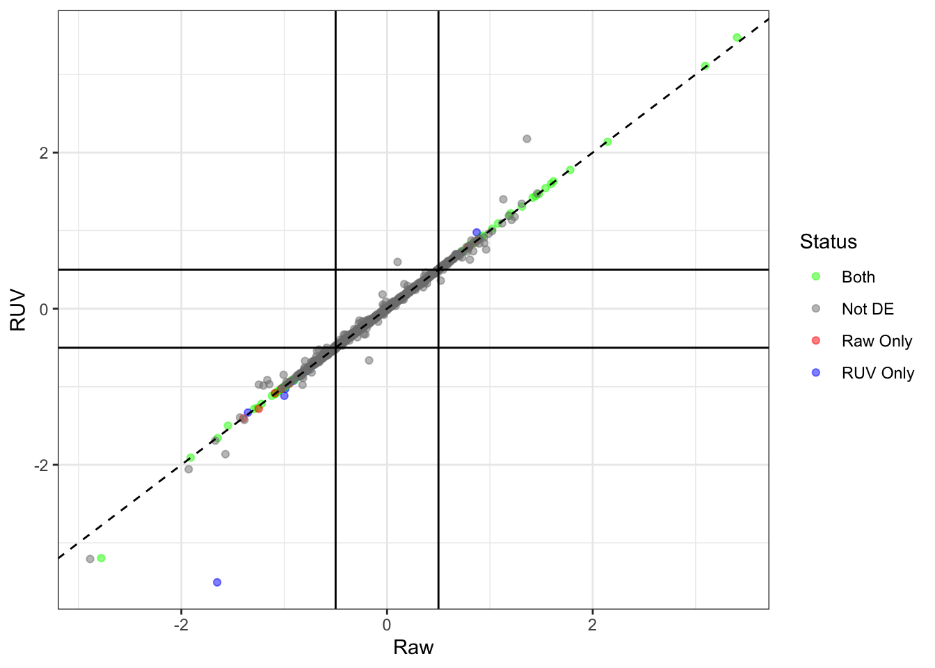
| Version | Author | Date |
|---|---|---|
| 6c61705 | yangdongau | 2020-02-27 |
The 228 genes considered as DE using an FDR of 0.01 and logFC beyond the range \(\pm 0.5\) were then inspected to confirm that the counts support their inclusion as DE.
Here plot CPM for DE genes having a FDR below 0.01 and logFC beyond the range \(\pm 1.2\)
ruv$normalizedCounts %>%
    cpm(log = TRUE) %>%
    .[dplyr::filter(topTable, FDR < 0.01 & abs(logFC) > 1.2)$ensembl_gene_id,] %>%
    as.data.frame() %>%
    rownames_to_column("ensembl_gene_id") %>%
    as_tibble() %>%
    gather(key = "sample", value = "CPM", -ensembl_gene_id) %>%
    left_join(dgeList$samples) %>%
    left_join(dgeList$genes) %>%
  ggplot(aes(Genotype, CPM)) +
  geom_point(aes(colour = Genotype)) +
  geom_line(
    aes(group = pair),
    colour = "grey70"
  ) +
  facet_wrap(~external_gene_name, scales = "free_y") +
    theme(legend.position = "none") +
  labs(y = "logCPM")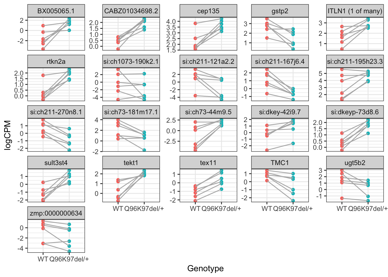
| Version | Author | Date |
|---|---|---|
| 6c61705 | yangdongau | 2020-02-27 |
Data Export
Final gene lists were exported as separate csv files, along with dgeList objects.
write.csv(topTableDE, here::here("output", "DEgenes.csv"))
write.csv(topTable,here::here("output", "topTable.csv"))
write_rds(dgeList, here::here("data", "dgeList.rds"), compress = "gz")
devtools::session_info()─ Session info ──────────────────────────────────────────────────────────
setting value
version R version 3.6.0 (2019-04-26)
os macOS Mojave 10.14.6
system x86_64, darwin15.6.0
ui X11
language (EN)
collate en_AU.UTF-8
ctype en_AU.UTF-8
tz Australia/Adelaide
date 2020-10-28
─ Packages ──────────────────────────────────────────────────────────────
package * version date lib source
annotate 1.62.0 2019-05-02 [1] Bioconductor
AnnotationDbi * 1.46.1 2019-08-20 [1] Bioconductor
AnnotationFilter * 1.8.0 2019-05-02 [1] Bioconductor
AnnotationHub * 2.16.0 2019-05-02 [1] Bioconductor
aroma.light 3.14.0 2019-05-02 [1] Bioconductor
assertthat 0.2.1 2019-03-21 [1] CRAN (R 3.6.0)
backports 1.1.4 2019-04-10 [1] CRAN (R 3.6.0)
Biobase * 2.44.0 2019-05-02 [1] Bioconductor
BiocFileCache * 1.8.0 2019-05-02 [1] Bioconductor
BiocGenerics * 0.30.0 2019-05-02 [1] Bioconductor
BiocManager 1.30.10 2019-11-16 [1] CRAN (R 3.6.0)
BiocParallel * 1.18.1 2019-08-06 [1] Bioconductor
biomaRt 2.40.4 2019-08-19 [1] Bioconductor
Biostrings * 2.52.0 2019-05-02 [1] Bioconductor
bit 1.1-14 2018-05-29 [1] CRAN (R 3.6.0)
bit64 0.9-7 2017-05-08 [1] CRAN (R 3.6.0)
bitops 1.0-6 2013-08-17 [1] CRAN (R 3.6.0)
blob 1.2.0 2019-07-09 [1] CRAN (R 3.6.0)
broom 0.5.2 2019-04-07 [1] CRAN (R 3.6.0)
callr 3.3.1 2019-07-18 [1] CRAN (R 3.6.0)
cellranger 1.1.0 2016-07-27 [1] CRAN (R 3.6.0)
cli 1.1.0 2019-03-19 [1] CRAN (R 3.6.0)
colorspace 1.4-1 2019-03-18 [1] CRAN (R 3.6.0)
crayon 1.3.4 2017-09-16 [1] CRAN (R 3.6.0)
curl 4.0 2019-07-22 [1] CRAN (R 3.6.0)
DBI 1.0.0 2018-05-02 [1] CRAN (R 3.6.0)
dbplyr * 1.4.2 2019-06-17 [1] CRAN (R 3.6.0)
DelayedArray * 0.10.0 2019-05-02 [1] Bioconductor
desc 1.2.0 2018-05-01 [1] CRAN (R 3.6.0)
DESeq 1.36.0 2019-05-02 [1] Bioconductor
devtools 2.2.2 2020-02-17 [1] CRAN (R 3.6.0)
digest 0.6.20 2019-07-04 [1] CRAN (R 3.6.0)
dplyr * 0.8.3 2019-07-04 [1] CRAN (R 3.6.0)
EDASeq * 2.18.0 2019-05-02 [1] Bioconductor
edgeR * 3.26.7 2019-08-13 [1] Bioconductor
ellipsis 0.3.0 2019-09-20 [1] CRAN (R 3.6.0)
ensembldb * 2.8.0 2019-05-02 [1] Bioconductor
evaluate 0.14 2019-05-28 [1] CRAN (R 3.6.0)
forcats * 0.4.0 2019-02-17 [1] CRAN (R 3.6.0)
fs 1.3.1 2019-05-06 [1] CRAN (R 3.6.0)
genefilter 1.66.0 2019-05-02 [1] Bioconductor
geneplotter 1.62.0 2019-05-02 [1] Bioconductor
generics 0.0.2 2018-11-29 [1] CRAN (R 3.6.0)
GenomeInfoDb * 1.20.0 2019-05-02 [1] Bioconductor
GenomeInfoDbData 1.2.1 2019-07-25 [1] Bioconductor
GenomicAlignments * 1.20.1 2019-06-18 [1] Bioconductor
GenomicFeatures * 1.36.4 2019-07-09 [1] Bioconductor
GenomicRanges * 1.36.0 2019-05-02 [1] Bioconductor
ggplot2 * 3.2.1 2019-08-10 [1] CRAN (R 3.6.0)
ggrepel * 0.8.1 2019-05-07 [1] CRAN (R 3.6.0)
git2r 0.26.1 2019-06-29 [1] CRAN (R 3.6.0)
glue 1.3.1 2019-03-12 [1] CRAN (R 3.6.0)
gtable 0.3.0 2019-03-25 [1] CRAN (R 3.6.0)
haven 2.1.1 2019-07-04 [1] CRAN (R 3.6.0)
here 0.1 2017-05-28 [1] CRAN (R 3.6.0)
highr 0.8 2019-03-20 [1] CRAN (R 3.6.0)
hms 0.5.1 2019-08-23 [1] CRAN (R 3.6.0)
htmltools 0.3.6 2017-04-28 [1] CRAN (R 3.6.0)
httpuv 1.5.1 2019-04-05 [1] CRAN (R 3.6.0)
httr 1.4.1 2019-08-05 [1] CRAN (R 3.6.0)
hwriter 1.3.2 2014-09-10 [1] CRAN (R 3.6.0)
interactiveDisplayBase 1.22.0 2019-05-02 [1] Bioconductor
IRanges * 2.18.2 2019-08-24 [1] Bioconductor
jsonlite 1.6 2018-12-07 [1] CRAN (R 3.6.0)
knitr 1.24 2019-08-08 [1] CRAN (R 3.6.0)
labeling 0.3 2014-08-23 [1] CRAN (R 3.6.0)
later 0.8.0 2019-02-11 [1] CRAN (R 3.6.0)
lattice 0.20-38 2018-11-04 [1] CRAN (R 3.6.0)
latticeExtra 0.6-28 2016-02-09 [1] CRAN (R 3.6.0)
lazyeval 0.2.2 2019-03-15 [1] CRAN (R 3.6.0)
limma * 3.40.6 2019-07-26 [1] Bioconductor
locfit 1.5-9.1 2013-04-20 [1] CRAN (R 3.6.0)
lubridate 1.7.4 2018-04-11 [1] CRAN (R 3.6.0)
magrittr * 1.5 2014-11-22 [1] CRAN (R 3.6.0)
MASS 7.3-51.4 2019-03-31 [1] CRAN (R 3.6.0)
Matrix 1.2-17 2019-03-22 [1] CRAN (R 3.6.0)
matrixStats * 0.54.0 2018-07-23 [1] CRAN (R 3.6.0)
memoise 1.1.0 2017-04-21 [1] CRAN (R 3.6.0)
mgcv 1.8-28 2019-03-21 [1] CRAN (R 3.6.0)
mime 0.7 2019-06-11 [1] CRAN (R 3.6.0)
modelr 0.1.5 2019-08-08 [1] CRAN (R 3.6.0)
munsell 0.5.0 2018-06-12 [1] CRAN (R 3.6.0)
nlme 3.1-141 2019-08-01 [1] CRAN (R 3.6.0)
pander * 0.6.3 2018-11-06 [1] CRAN (R 3.6.0)
pillar 1.4.2 2019-06-29 [1] CRAN (R 3.6.0)
pkgbuild 1.0.6 2019-10-09 [1] CRAN (R 3.6.0)
pkgconfig 2.0.2 2018-08-16 [1] CRAN (R 3.6.0)
pkgload 1.0.2 2018-10-29 [1] CRAN (R 3.6.0)
prettyunits 1.0.2 2015-07-13 [1] CRAN (R 3.6.0)
processx 3.4.1 2019-07-18 [1] CRAN (R 3.6.0)
progress 1.2.2 2019-05-16 [1] CRAN (R 3.6.0)
promises 1.0.1 2018-04-13 [1] CRAN (R 3.6.0)
ProtGenerics 1.16.0 2019-05-02 [1] Bioconductor
ps 1.3.0 2018-12-21 [1] CRAN (R 3.6.0)
purrr * 0.3.3 2019-10-18 [1] CRAN (R 3.6.0)
R.methodsS3 1.7.1 2016-02-16 [1] CRAN (R 3.6.0)
R.oo 1.22.0 2018-04-22 [1] CRAN (R 3.6.0)
R.utils 2.9.0 2019-06-13 [1] CRAN (R 3.6.0)
R6 2.4.0 2019-02-14 [1] CRAN (R 3.6.0)
rappdirs 0.3.1 2016-03-28 [1] CRAN (R 3.6.0)
RColorBrewer 1.1-2 2014-12-07 [1] CRAN (R 3.6.0)
Rcpp 1.0.2 2019-07-25 [1] CRAN (R 3.6.0)
RCurl 1.95-4.12 2019-03-04 [1] CRAN (R 3.6.0)
readr * 1.3.1 2018-12-21 [1] CRAN (R 3.6.0)
readxl 1.3.1 2019-03-13 [1] CRAN (R 3.6.0)
remotes 2.1.1 2020-02-15 [1] CRAN (R 3.6.0)
rlang 0.4.4 2020-01-28 [1] CRAN (R 3.6.0)
rmarkdown 1.15 2019-08-21 [1] CRAN (R 3.6.0)
rprojroot 1.3-2 2018-01-03 [1] CRAN (R 3.6.0)
Rsamtools * 2.0.0 2019-05-02 [1] Bioconductor
RSQLite 2.1.2 2019-07-24 [1] CRAN (R 3.6.0)
rstudioapi 0.10 2019-03-19 [1] CRAN (R 3.6.0)
rtracklayer 1.44.3 2019-08-24 [1] Bioconductor
RUVSeq * 1.18.0 2019-05-02 [1] Bioconductor
rvest 0.3.4 2019-05-15 [1] CRAN (R 3.6.0)
S4Vectors * 0.22.0 2019-05-02 [1] Bioconductor
scales * 1.0.0 2018-08-09 [1] CRAN (R 3.6.0)
sessioninfo 1.1.1 2018-11-05 [1] CRAN (R 3.6.0)
shiny 1.3.2 2019-04-22 [1] CRAN (R 3.6.0)
ShortRead * 1.42.0 2019-05-02 [1] Bioconductor
stringi 1.4.3 2019-03-12 [1] CRAN (R 3.6.0)
stringr * 1.4.0 2019-02-10 [1] CRAN (R 3.6.0)
SummarizedExperiment * 1.14.1 2019-07-31 [1] Bioconductor
survival 2.44-1.1 2019-04-01 [1] CRAN (R 3.6.0)
testthat 2.3.1 2019-12-01 [1] CRAN (R 3.6.0)
tibble * 2.1.3 2019-06-06 [1] CRAN (R 3.6.0)
tidyr * 0.8.3 2019-03-01 [1] CRAN (R 3.6.0)
tidyselect 0.2.5 2018-10-11 [1] CRAN (R 3.6.0)
tidyverse * 1.2.1 2017-11-14 [1] CRAN (R 3.6.0)
usethis 1.5.1 2019-07-04 [1] CRAN (R 3.6.0)
vctrs 0.2.0 2019-07-05 [1] CRAN (R 3.6.0)
whisker 0.4 2019-08-28 [1] CRAN (R 3.6.0)
withr 2.1.2 2018-03-15 [1] CRAN (R 3.6.0)
workflowr 1.6.0 2019-12-19 [1] CRAN (R 3.6.0)
xfun 0.9 2019-08-21 [1] CRAN (R 3.6.0)
XML 3.98-1.20 2019-06-06 [1] CRAN (R 3.6.0)
xml2 1.2.2 2019-08-09 [1] CRAN (R 3.6.0)
xtable 1.8-4 2019-04-21 [1] CRAN (R 3.6.0)
XVector * 0.24.0 2019-05-02 [1] Bioconductor
yaml 2.2.0 2018-07-25 [1] CRAN (R 3.6.0)
zeallot 0.1.0 2018-01-28 [1] CRAN (R 3.6.0)
zlibbioc 1.30.0 2019-05-02 [1] Bioconductor
[1] /Library/Frameworks/R.framework/Versions/3.6/Resources/library